Categories
General

Response to PRA DP3/21

The PRA have issued Discussion Paper DP3/21 consulting on changes to the PRA Rulebook. All the changes discussed seem very sensible and we support them, in particular integrating Supervisory Statements with the Rulebook. Our formal response is below.

Categories
FSMA R

Extracting data from PDF files using R

Purpose

This post illustrates how R can be used to extract numerical information from PDF files. The technique is illustrated by extracting the Credit Risk Premium and Valuation Uncertainty parameters from the PDF file containing the instructions for the PRA’s 2021 Solvency II Quantitative Impact Study (QIS).

(Note that since this post was written, the PRA have updated the QIS instructions. This has changed the pagination of the PDF file slightly. The code below has not been updated for this.)

This post is partly to illustrate how to extract data from PDF files, and partly preparation for a later one discussing the QIS in more detail, in particular the draft redesign of the Fundamental Spread. See this post for a general introduction to the existing Fundamental Spread.

Introduction

PDF stands for Portable Document Format. This format is designed for presentation, principally to look the same on-screen as when printed out, and so some work is needed to extract data from it.

Copying and pasting tables from PDF files into Word or Excel often does not work very well and needs manual adjustment, for example using Excel’s Convert Text to Columns feature.

The R library pdftools reads PDF files and does a great deal of work behind the scenes to represent their content as text, which provides an alternative to copying from a PDF viewer.

Using R is more auditable than manually copying/pasting, because all the code used is stored for later examination (it can be thought of as a ‘recording’ of the manipulation). Being code-based, it can in principle be automated for use-cases where PDFs in the same overall format are regularly updated (this does not apply to the QIS case study, but the point holds in general).

Download and open the PDF file

The calibrations tested in the PRA QIS are included in the ‘instructions’ PDF file at: https://www.bankofengland.co.uk/-/media/boe/files/prudential-regulation/solvency-ii/solvency-ii-reform-quantitative-impact-survey/qis-instructions.pdf.

The instructions file is downloaded to the working directory using R as follows. Note that the mode must be set to "wb" on Windows to download as a binary file, to avoid file corruption issues from treating it as text.

url <- "https://www.bankofengland.co.uk/-/media/boe/files/prudential-regulation/solvency-ii/solvency-ii-reform-quantitative-impact-survey/qis-instructions.pdf"
pdf_file <- "qis-instructions.pdf"
download.file(url, pdf_file, mode = "wb")

First we use the pdftools::pdf_info function to look at some basic information:

pdf_i <- pdftools::pdf_info(pdf_file)

# Page count
pdf_i$pages
#> [1] 35

# Author, Producer, Title
pdf_i$keys
#> $Author
#> [1] "Prudential Regulation Authority, Bank of England"
#> 
#> $Producer
#> [1] "Microsoft: Print To PDF"
#> 
#> $Title
#> [1] "Review of Solvency II - QIS Instructions"

All is as expected, so we can now load the PDF file in full using pdftools::pdf_text. This returns an R character vector with one entry per page (so 35 entries since there are 35 pages as noted above). Each page is a continuous stream of text, with embedded newlines ("\n" in R).

pdf_pages <- pdftools::pdf_text(pdf_file)
str(pdf_pages)
#>  chr [1:35] "Review of Solvency II 㤼㸶 Quantitative Impact Study (QIS)\nInstructions for completing the QIS template(s)\n\nVer"| __truncated__ ....

Extract the Credit Risk Premium parameters

From looking at the file in a PDF viewer, the credit risk premium (CRP) parameters are on page 28. We use cat to view this page with newlines shown as such, rather than "\n". It can be seen that the ‘text’ version of the PDF provided by pdftools is reasonably faithful to the original, with the embedded tables laid out logically, and so it will be possible to extract the numerical values.

cat(pdf_pages[[28]])
#>       (ii) A percentage applied to the 5-year average spread on an index of the same sector
#>            and CQS as the asset.
#> 
#> 10. The percentages to be used in 9(i) and 9(ii) are as follows:
#> 
#>                                                               Scenario A                  Scenario B
#>  Percentage applied to current z-spread                            25%                        25%
#>  Percentage applied to average spread                              25%                         0%
#> 
#> 11. The 5-year average spreads to be used for the purposes of 9(ii) above are as follows:
#> 
#>                    5-year average spreads (bps)
#>                Financials            Non-Financials
#>      CQS 0           90                       79
#>      CQS 1          121                      112
#>      CQS 2          180                      159
#>      CQS 3          276                      197
#>      CQS 4          462                      379
#>      CQS 5          693                      656
#>      CQS 6          693                      656
#> 
#> 12. For the purposes of this QIS, we will be testing both a floor and a cap applied to the total
#>     CRP. The floor will be applied in Scenarios A and B and all the sensitivities tested under
#>     them. The cap will be tested both on and off in Scenario A only19. The following table
#>     sets out the floor and cap to be applied to the total CRP.
#> 
#>                  CRP floor for Scenario A and B
#>                                                                  CRP cap for Scenario A (bps)
#>                               (bps)
#>                   Financials      Non-Financials                  Financials         Non-Financials
#>      CQS 0               11                      4                     56                    42
#>      CQS 1               27                      19                   101                    86
#>      CQS 2               43                      28                   153                    124
#>      CQS 3               72                      40                   229                    166
#>      CQS 4              168                     117                   507                    403
#>      CQS 5              391                     184                  1,037                   623
#>      CQS 6              391                     184                  1,207                   793
#> 
#> 13. The following table summarises the scenarios in which the floor and cap should be
#>     applied.
#> 
#> 19 As stated above, there are a number of cells in Scenario A of the template with the explicit direction that figures
#> are to be provided on the basis of a cap being applied. Unless such explicit direction is give, please provide
#> figures on the basis that the cap is not applied.
#> 
#> 28

The text representation isn’t perfect – footnote 19 is not shown in superscript, for example – but it’s definitely usable.

To ease parsing page 28, we use strsplit to break the text up by newlines, so we can read each line individually. For example lines 6 to 8 hold the CRP percentages to apply to z-spreads in each scenario, lines 13 to 20 hold the 5-year average spreads, and lines 30-37 hold the floors and caps:

p28_lines <- strsplit(pdf_pages[[28]], "\n")[[1]] # strsplit returns a 1-item list here and we want the first item itself

# Percentages
p28_lines[6:8]
#> [1] "                                                              Scenario A                  Scenario B"
#> [2] " Percentage applied to current z-spread                            25%                        25%"   
#> [3] " Percentage applied to average spread                              25%                         0%"

# 5-year average spreads
p28_lines[13:20]
#> [1] "               Financials            Non-Financials"
#> [2] "     CQS 0           90                       79"   
#> [3] "     CQS 1          121                      112"   
#> [4] "     CQS 2          180                      159"   
#> [5] "     CQS 3          276                      197"   
#> [6] "     CQS 4          462                      379"   
#> [7] "     CQS 5          693                      656"   
#> [8] "     CQS 6          693                      656"

# Floors and caps
p28_lines[27:37]
#>  [1] "                 CRP floor for Scenario A and B"                                                    
#>  [2] "                                                                 CRP cap for Scenario A (bps)"      
#>  [3] "                              (bps)"                                                                
#>  [4] "                  Financials      Non-Financials                  Financials         Non-Financials"
#>  [5] "     CQS 0               11                      4                     56                    42"    
#>  [6] "     CQS 1               27                      19                   101                    86"    
#>  [7] "     CQS 2               43                      28                   153                    124"   
#>  [8] "     CQS 3               72                      40                   229                    166"   
#>  [9] "     CQS 4              168                     117                   507                    403"   
#> [10] "     CQS 5              391                     184                  1,037                   623"   
#> [11] "     CQS 6              391                     184                  1,207                   793"

Now we need to pull out the numbers. This is hardly worth doing for the percentages, which could just be typed in, but it establishes the general principle we’ll use for the other tables.

The idea is to use regular expressions to search for numerical values systematically. The regular expression [0-9] means ‘a digit character’ and the "+" means ‘one or more of’. Thus [0-9]+ will match a sequence of digits of any length. This is sufficient to parse the percentages, but to deal with embedded commas and decimal points in later tables, we expand it to [0-9,\\.]+, which means one or more of (1) a digit character (2) a comma and (3) a decimal point.

The decimal point is a ‘special’ character for regular expressions that matches anything, so we have to precede it with a \ character, and in turn this has to be doubled for R to recognise it as a \. The power of regular expressions makes it worthwhile to tolerate these fiddly subtleties!

This isn’t a fully general way of parsing numbers, but it suffices for the PRA QIS tables here.

We wrap this into a function parse_numbers that matches the numerical text, deals with embedded commas, converts the results to numbers while retaining the embedded decimal points, and arranges the results as a matrix.

Enclosing this regular expression in parentheses means ‘capture anything matching this expression’, and the combination of gregexpr and regmatches captures the matching expressions and discards the non-matching text.

For simplicity we add the row and column names manually rather than by parsing.

parse_numbers <- function(text_lines) {
  matches <- regmatches(text_lines, gregexpr("([0-9,\\.]+)", text_lines))
  matches <- t(simplify2array(matches)) # t to transpose the result of simplify2array
  nr <- nrow(matches) # Keep the number of rows so it can be restored later
  matches <- gsub(",", "", matches) # Remove commas
  matches <- matrix(as.numeric(matches), nrow = nr) # Convert to actual numbers rather than text representing numbers
  return(matches)
}

crp_fac <- parse_numbers(p28_lines[7:8]) / 100 # Convert to numerically correct rather than percentages
rownames(crp_fac) <- c("Current", "5yrAverage")
colnames(crp_fac) <- c("ScenarioA", "ScenarioB")
crp_fac
#>            ScenarioA ScenarioB
#> Current         0.25      0.25
#> 5yrAverage      0.25      0.00

We use parse_numbers again to pull out the 5-year average spreads, and put these in a data frame labelled with the CQSs in the first column:

crp_5yr_avg_bp <- as.data.frame(parse_numbers(p28_lines[14:20]))
crp_5yr_avg_bp[,1] <- paste0("CQS", crp_5yr_avg_bp[,1])
colnames(crp_5yr_avg_bp) <- c("CQS", "Financial", "NonFinancial")
crp_5yr_avg_bp
#>    CQS Financial NonFinancial
#> 1 CQS0        90           79
#> 2 CQS1       121          112
#> 3 CQS2       180          159
#> 4 CQS3       276          197
#> 5 CQS4       462          379
#> 6 CQS5       693          656
#> 7 CQS6       693          656

Finally we pull out the CRP floors and caps, which are laid out as a 5-column table, and split this into two separate data frames:

crp_floor_cap_bp <- as.data.frame(parse_numbers(p28_lines[31:37]))
crp_floor_cap_bp[,1] <- paste0("CQS", crp_floor_cap_bp[,1])
crp_floor_bp <- crp_floor_cap_bp[,1:3]
crp_cap_bp <- crp_floor_cap_bp[,c(1, 4:5)]

colnames(crp_floor_bp) <- colnames(crp_cap_bp) <- c("CQS", "Financial", "NonFinancial")
crp_floor_bp
#>    CQS Financial NonFinancial
#> 1 CQS0        11            4
#> 2 CQS1        27           19
#> 3 CQS2        43           28
#> 4 CQS3        72           40
#> 5 CQS4       168          117
#> 6 CQS5       391          184
#> 7 CQS6       391          184

crp_cap_bp
#>    CQS Financial NonFinancial
#> 1 CQS0        56           42
#> 2 CQS1       101           86
#> 3 CQS2       153          124
#> 4 CQS3       229          166
#> 5 CQS4       507          403
#> 6 CQS5      1037          623
#> 7 CQS6      1207          793

Extract Valuation Uncertainty parameters

The Valuation Uncertainty (VU) parameters are on page 29.

p29_lines <- strsplit(pdf_pages[[29]], "\n")[[1]]

# VU parameters
p29_lines[19:24]
#> [1] "         CQS                  IFRS Level            VU for Scenario A            VU for Scenario B"
#> [2] "                                                          (bps)                        (bps)"      
#> [3] "          All                   Level 1                    NIL                           Nil"      
#> [4] "          All                   Level 2                     7.5                         3.75"      
#> [5] "          0-3                   Level 3                     7.5                         3.75"      
#> [6] "          4-6                   Level 3                    25.0                        12.50"

We pull these out, omitting the row for IFRS Level 1 since this complicates the parsing, and starting the parse at character 30 to omit the CQS column which will otherwise confuse matters.

We then add in the CQS column, manually expand the rows to refer to CQS explicitly, and include zero values for IFRS level 1 at the top.

vu_lines <- p29_lines[22:24]
vu_lines <- unname(vapply(vu_lines, function(x) substr(x, 30, nchar(x)), character(1)))
ex_cqs_vu_bp <- as.data.frame(parse_numbers(vu_lines))
ex_cqs_vu_bp[,1] <- paste0("IFRS", ex_cqs_vu_bp[,1])
colnames(ex_cqs_vu_bp) <- c("IFRSLevel", "ScenarioA", "ScenarioB")
vu_bp <- rbind(data.frame(CQS = paste0("CQS", 0:6), data.frame(IFRSLevel = "IFRS1", ScenarioA = 0, ScenarioB = 0)),
               data.frame(CQS = paste0("CQS", 0:6), ex_cqs_vu_bp[1,]), # First row is IFRS2 all CQS
               data.frame(CQS = paste0("CQS", 0:3), ex_cqs_vu_bp[2,]), # Second row is IFRS3 CQS0-3
               data.frame(CQS = paste0("CQS", 4:6), ex_cqs_vu_bp[3,])) # Third row is IFRS3 CQS4-6
vu_bp
#>     CQS IFRSLevel ScenarioA ScenarioB
#> 1  CQS0     IFRS1       0.0      0.00
#> 2  CQS1     IFRS1       0.0      0.00
#> 3  CQS2     IFRS1       0.0      0.00
#> 4  CQS3     IFRS1       0.0      0.00
#> 5  CQS4     IFRS1       0.0      0.00
#> 6  CQS5     IFRS1       0.0      0.00
#> 7  CQS6     IFRS1       0.0      0.00
#> 8  CQS0     IFRS2       7.5      3.75
#> 9  CQS1     IFRS2       7.5      3.75
#> 10 CQS2     IFRS2       7.5      3.75
#> 11 CQS3     IFRS2       7.5      3.75
#> 12 CQS4     IFRS2       7.5      3.75
#> 13 CQS5     IFRS2       7.5      3.75
#> 14 CQS6     IFRS2       7.5      3.75
#> 15 CQS0     IFRS3       7.5      3.75
#> 16 CQS1     IFRS3       7.5      3.75
#> 17 CQS2     IFRS3       7.5      3.75
#> 18 CQS3     IFRS3       7.5      3.75
#> 19 CQS4     IFRS3      25.0     12.50
#> 20 CQS5     IFRS3      25.0     12.50
#> 21 CQS6     IFRS3      25.0     12.50

Save the parameters

Finally we save the CRP and VU parameters to RDS (R format) and CSV (for Excel) files for later analysis.

saveRDS(crp_fac, "qis21_crp_fac.rds")
saveRDS(crp_5yr_avg_bp, "qis21_crp_5yr_avg_bp.rds")
saveRDS(crp_floor_bp, "qis21_crp_floor_bp.rds")
saveRDS(crp_cap_bp, "qis21_crp_cap_bp.rds")
saveRDS(vu_bp, "qis21_vu_bp.rds")

write.csv(crp_fac, "qis21_crp_fac.csv", row.names = FALSE)
write.csv(crp_5yr_avg_bp, "qis21_crp_5yr_avg_bp.csv", row.names = FALSE)
write.csv(crp_floor_bp, "qis21_crp_floor_bp.csv", row.names = FALSE)
write.csv(crp_cap_bp, "qis21_crp_cap_bp.csv", row.names = FALSE)
write.csv(vu_bp, "qis21_vu_bp.csv", row.names = FALSE)

Summary

In this post, we showed how the R package pdftools and R’s built-in regular expressions capability can be used to pull numerical information out of PDF files.

Categories
FSMA Solvency II

Response to HMT Call for Evidence on Solvency II

Our response to the HMT Call for Evidence is available here. The executive summary is reproduced below for ease of reference.

A more transparent and principles-based regime

In the current Solvency II regime, there is a substantial degree of disconnection between what things mean and how they are calculated. For example, as the Call for Evidence notes, it is generally accepted that the method by which the Risk Margin (RM) is calculated does not lead to a sensible outcome in relation to its intended meaning, both in relation to the size of the RM and its volatility in response to changes in interest rates. Similar effects apply in relation to the Matching Adjustment as discussed later in this note. The Call for Evidence rightly identifies an opportunity to rebalance the mix of rules and judgement.

This is likely to result in the PRA having more powers, both formally (through changes to legislation or the PRA Rulebook), and informally through a greater degree of establishing and interpreting principles and exercising judgement. This increase in powers should be balanced by an increase in transparency, so that the firms the PRA regulates and supervises understand the reasoning behind the PRA’s expectations and where appropriate are able to challenge the PRA’s judgements effectively.

As part of improving transparency, key aspects of the regime should be better defined, for example by explaining what an element is intended to represent in terms of a risk appetite or confidence level. The SCR is well-defined in these terms (99.5% confidence over 1 year), but the same cannot be said of the Fundamental Spread, where in the current regime the level of confidence relating to long-term default and downgrade risk is an opaque consequence of the methodology used to calculate it. This opacity is unhelpful, for example it makes it difficult to ensure that different asset classes are being treated in an equivalent way.

Risk Margin

We agree with the diagnosis in the Call for Evidence of the issues with the RM. The issues are sufficiently serious that technocratic adjustment to the calculation methodology (for example the ‘lambda factors’ recently proposed by EIOPA[1]) is insufficient and a more fundamental reform is needed.

The MOCE concept introduced by IAIS[2] appears to be more sensibly designed than the RM and is based on well-defined confidence levels for life and general insurers. Aligning with IAIS would have obvious practical benefits for firms that will become subject to IAIS in due course.

Matching Adjustment

We support the economic rationale for allowing a mechanism like the MA. As the Call for Evidence notes, there are many benefits from the MA. However, there are pros and cons to any such regime. We consider the MA regime needs to be revised to improve outcomes for policyholders, firms, the PRA, and the UK economy.

The MA should be regarded by firms as a privilege, not a right. Both firms and the PRA should approach the MA with an appropriate degree of humility, as it relies on accurate risk measurement over long time horizons.

We consider the definition of the MA as an adjustment to liability valuation to be unhelpful. In our view, it is better to frame the Matching Adjustment as a way of recognising the risk-mitigating effects of a credible hold-to-maturity strategy. It should be shown as a separate item on the asset side of the balance sheet, arising from a synergy between the assets and liabilities and depending on both, but not directly part of the valuation of either. In this framing, the investment assets and insurance liabilities both remain at market / market-consistent values. The separate MA asset would recognise the risk-mitigating effect of the hold-to-maturity strategy on the regulatory balance sheet, net of all relevant risks, including but not limited to those measured by the current FS. This framing more clearly expresses what the concept means, rather than how it is calculated (via an addition to the liability discount rate).

The MA relies on separation of credit from non-credit risk. This is technically challenging, and impossible to achieve with complete confidence. There is a risk of falling into a ‘best is the enemy of the good’ trap here: lower annuity prices, more long-term investment and reduced procyclicality are all very worthwhile outcomes, and our view is that these outcomes merit accepting some degree of uncertainty over the measurement of credit risk. The balance to be struck is a risk appetite question for HMT and the PRA.

The credit-riskiness of the cashflows is not the only risk. All risks to the credibility of a hold-to-maturity strategy need to be considered, either through measurement (in the equivalent of the FS) or exclusion (the eligibility criteria). The presentation of the MA as an asset rather than an addition to the discount rate enables the equivalent of the FS to be composed of different monetary reserves. This is a more general lens through which to examine the allowance for risks and facilitates a more flexible approach than either excluding risks entirely or forcing them through the FS as a basis points item. We believe it would then be possible (within reason) to relax eligibility criteria around cashflow fixity, prepayment risk and cashflow matching by introducing compensation for these risks within an expanded definition of the FS.

The current FS is based on a complex, inelegant, and internally inconsistent methodology inherited by the PRA from EIOPA. In our view, the definition of the credit element of the FS (as distinct from prepayment and mismatching elements) should be recast as:

  • a best-estimate allowance for all relevant risks impacting on asset cashflows; plus
  • an additional well-defined allowance for risk, which could be considered as a ‘credit risk premium’.

The allowance for the credit risk premium should be based on a well-defined risk appetite articulated by HMT or the PRA, with a transparent and detailed methodology giving effect to this risk appetite published by the PRA so that interested parties can scrutinise and challenge the calibration against this appetite. This risk appetite would in effect express the balance struck between the trade-offs embedded in the use of the ALMA concept, reflecting costs, benefits and risks to policyholders and wider society.

The overall calibration of the expanded FS is again a risk appetite question for HMT and the PRA, within the design considerations outlined above. The balance between using credit ratings and market prices needs to be reconsidered: the MA regime essentially gives almost no weight to current market prices as a source of information on credit risk, other than in the special case of the BBB cliff in Article 77c(1)(c) of the Solvency II Framework Directive. The focus on credit ratings has a very strong stabilising effect, arguably excessively so: in our view this needs to be rebalanced towards giving some weight to market prices alongside credit ratings. Again, this is primarily a risk appetite question, as it bears on the cost/benefit trade-off from the MA.

In the current MA regime, we believe there is more strength in the SCR than on the base balance sheet. This balance should be reconsidered: we believe it would be better to have more strength in base than the current FS, particularly for internally rated assets, and a corresponding reduction in the SCR – when the base is stronger, there is less risk to be covered by the SCR. While there would be a loss of diversification benefit from reducing the SCR, there would also be a reduction in the capital buffers firms hold on top of the SCR and the impact might reasonably be broadly neutral overall.

Solvency Capital Requirement

The distinction between the Standard Formula and (partial) Internal Models is too hard-edged and more flexibility is needed. This should include:

  • More granularity in the risk modules – for example at present credit risk is ‘all or nothing’ and it would be beneficial to some firms to be able to use the SF for corporate bonds while having an internal model for risks where the SF was inappropriate. This would be a more proportionate approach for small firms with specialised exposures.
  • Widening the scope of undertaking-specific parameters (USPs), in particular to include asset risks. This would enable customisation within a predefined methodology for asset classes other than corporate bonds, and act as a helpful half-way house between the SF and a full IM.

There is limited transparency in the calibration of the SF at present. The PRA should improve this on a gradual basis starting with the most material risks. This would also have the benefit of improving the transparency of the PRA’s Quantitative Indicator (QI) framework[3]: if the historical circumstances had been such that the PRA had adopted its own view for SF purposes there would be no need to have distinct IM QIs for the same risks, although some QIs would still need to be adapted to fit the risk profile of each firm applying for an IM.

The PRA should have powers to adjust Technical Provisions directly (in the manner of a ‘capital resources add-on’ under the prior UK ICAS regime) rather than using an adjustment to the SCR to achieve the same effect. The PRA should be accountable for the use of this power via existing mechanisms, including being subject to the Tribunal, and should also disclose aggregate statistics on how often it is used.


[1] See page 30 of EIOPA’s Opinion on the 2020 Review of Solvency II at https://www.eiopa.europa.eu/content/opinion-2020-review-of-solvency-ii_en

[2] See section 5.3 of Public 2020 ICS Data Collection Technical Specifications at https://www.iaisweb.org/page/supervisory-material/insurance-capital-standard/file/90757/public-2020-ics-data-collection-technical-specifications

[3] See the 2016 letter from Sam Woods (then in his capacity of Executive Director of PRA Insurance Supervision) at https://www.bankofengland.co.uk/-/media/boe/files/prudential-regulation/letter/2016/sam-woods-reflections-2015-solvency-ii-internal-model-approval-process-jan-2016.pdf

Categories
FSMA R

Plotting the EIOPA Fundamental Spread Tables

Purpose

This post illustrates how EIOPA’s corporate bond Fundamental Spread tables can be visualised using R. It is structured as follows:

  • We introduce the Fundamental Spread, its structure and granularity.
  • Then we use the R openxlsx library to extract selected FS tables from the workbook published by EIOPA at 31 December 2019, and the tidyr library to manipulate this into a more congenial format.
  • Finally we use the ggplot2 library to produce plots of the FS.

Introduction

In Solvency II, the Fundamental Spread (FS) is the part of a bond’s spread that is treated as compensating for the cost of defaults and downgrades. The remaining yield is available as Matching Adjustment (MA). Insurers with the relevant regulatory approval can capitalise the MA by adding it to the basic risk-free rate and thereby reduce the value of their best-estimate liabilities.

The FS is measured in spread terms (presented for example as basis points). There are two different calibrations, one for corporate bonds, and the other for central government and central bank bonds.

For corporate bonds, the FS is:

  • the cost of default, confusingly denoted PD even though it is an expected loss and not a probability of default
  • plus cost of downgrades (CoD)
  • with the total being subject to a floor of 35% of long-term average spreads (LTAS) to swaps.

There is a second kind of PD (sometimes called PD-prob). This is actually a probability of default, and is combined with a recovery rate of 30% to give cashflow risk-adjustment factors. The two PDs are not derived in a completely consistent manner with each other and the basis points equivalent of the PD-prob combined with the recovery rate is close to but not identical with the PD element of the FS.

The corporate bond FS varies by:

  • currency: values for many global currencies are produced, including EUR, GBP and USD
  • sector: financial or non-financial
  • Credit Quality Step (CQS), a mapped credit rating, from CQS0 to CQS6
  • cashflow maturity (sometimes confusingly called duration in the regulations)

For completeness, we note that for government bonds, PD (both kinds) and CoD are zero, and the FS is a proportion of the LTAS to swaps. For EU member states, the proportion is 30% and for other states it is 35%. Negative FS values are set to zero. And the government bond FS varies by:

  • country (not currency – central government bond LTAS for different countries within the Eurozone are markedly different)
  • cashflow tenor

Data acquisition and processing

The FS is published by EIOPA as a set of tables within an Excel workbook held in a zip file. The zip file for 31 December 2019 is at https://www.eiopa.europa.eu/sites/default/files/risk_free_interest_rate/eiopa_rfr_20191231_0_0.zip.

This is downloaded and unzipped in the working directory using R as follows:

url <- "https://www.eiopa.europa.eu/sites/default/files/risk_free_interest_rate/eiopa_rfr_20191231_0_0.zip"
zip_file <- "eiopa_rfr_20191231_0_0.zip"
download.file(url, zip_file)
utils::unzip(zip_file)

There are four Excel files extracted from the zip file:

list.files(pattern = "xlsx$")

#> [1] "EIOPA_RFR_20191231_PD_Cod.xlsx"         
#> [2] "EIOPA_RFR_20191231_Qb_SW.xlsx"          
#> [3] "EIOPA_RFR_20191231_Term_Structures.xlsx"
#> [4] "EIOPA_RFR_20191231_VA_portfolios.xlsx"

We want the one with PD_Cod in its name, and load this in using loadWorkbook as follows:

xlsx_file <- "EIOPA_RFR_20191231_PD_Cod.xlsx"
wkb <- openxlsx::loadWorkbook(xlsx_file)

We now have an object wkb that represents the workbook in R. Readers familiar with VBA can think of this as being somewhat like a Workbook object, although the functionality available in the R openxlsx library is much more limited than in VBA. As a very basic example of using openxlsx, we can see the sheet names in R by calling names on the workbook object:

names(wkb)

#>  [1] "Main"           "LTAS_Govts"     "TM_Info"        "LTAS_Corps"    
#>  [5] "LTAS_Basic_RFR" "LTAS_Specifics" "FS_Govts"       "EUR"           
#>  [9] "BGN"            "HRK"            "CZK"            "DKK"           
#> [13] "HUF"            "LIC"            "PLN"            "NOK"           
#> [17] "RON"            "RUB"            "SEK"            "CHF"           
#> [21] "GBP"            "AUD"            "BRL"            "CAD"           
#> [25] "CLP"            "CNY"            "COP"            "HKD"           
#> [29] "INR"            "JPY"            "MYR"            "MXN"           
#> [33] "NZD"            "SGD"            "ZAR"            "KRW"           
#> [37] "TWD"            "THB"            "TRY"            "USD"           
#> [41] "ECB_reconst"

Examination of the downloaded workbook in Excel shows that the corporate bond FSs are on sheets named by currency, for example GBP. There are eight blocks of data for corporate bond FSs, four for financial-sector bonds, and four more for the non-financial sector. The four blocks in each sector are:

  • the PD-prob (to be combined with the recovery rate to give cashflow risk-adjustment factors)
  • the PD element of the FS
  • the total FS
  • the CoD element of the FS

Each block has 31 rows (a header plus 30 maturities) and 8 columns (a header plus 7 CQSs).

The readWorkbook function reads cells from a workbook object (here wkb). Since we are going to read in multiple blocks of data of the same size and shape, it makes sense to write a small helper function to read in a block first, fix up the column headings and keep track of what the block represents.

We test this out on the first block, which starts in row 10 column 2 (cell B10).

read_fs_block <- function(wkb, sheet, start_row, start_col, item, sector, scalar, row_size = 31, col_size = 8) {
  rows_to_read <- start_row:(start_row + row_size - 1)
  cols_to_read <- start_col:(start_col + col_size - 1)
  res <- openxlsx::readWorkbook(wkb, sheet, startRow = start_row, rows = rows_to_read, cols = cols_to_read)
  
  # EIOPA store the currency in the top-left, replace with maturity as that's what the column represents
  colnames(res)[1] <- "maturity"
  
  # Set up column names starting with CQS
  colnames(res)[2:col_size] <- paste0("CQS", colnames(res)[2:col_size])
  
  # Apply the scalar to all columns but the first
  res[,2:col_size] <- res[,2:col_size] * scalar
  
  # Add columns to track what currency, item and sector this block is for
  res$currency <- sheet
  res$item <- item
  res$sector <- sector
  res <- res[c((col_size + 1):(col_size + 3), 1:col_size)] # Permute columns
  
  return(res)
}

# No need to scale pd_prob, but we will scale the items in % to convert them to basis points
test_block <- read_fs_block(wkb, "GBP", 10, 2, item = "pd_prob", sector = "Financial", scalar = 1)

knitr::kable(head(test_block), format = "html", table.attr = "class=\"kable\"") # Look at the first few rows

currency item sector maturity CQS0 CQS1 CQS2 CQS3 CQS4 CQS5 CQS6
GBP pd_prob Financial 1 0.0000000 0.0005000 0.0009000 0.0023000 0.0113000 0.0345000 0.1588000
GBP pd_prob Financial 2 0.0002734 0.0010666 0.0018983 0.0051388 0.0244878 0.0689617 0.2589408
GBP pd_prob Financial 3 0.0007281 0.0016994 0.0030082 0.0084572 0.0387772 0.1019684 0.3253810
GBP pd_prob Financial 4 0.0013110 0.0024005 0.0042404 0.0122032 0.0536319 0.1329282 0.3720985
GBP pd_prob Financial 5 0.0019908 0.0031736 0.0056027 0.0163285 0.0686840 0.1616724 0.4069709
GBP pd_prob Financial 6 0.0027496 0.0040226 0.0071008 0.0207871 0.0836817 0.1882396 0.4344784

We can now write a further helper function to read in all 8 blocks on a sheet and combine them. This function also manipulates the data to calculate the impact of the FS floor (i.e. the extent to which the FS is more than the sum of PD and CoD).

read_fs_blockset <- function(wkb, sheet) {
  # The spec is a data frame where each row describes where a block starts and what it means
  spec <- data.frame(
    start_row = c(10, 10, 10, 10, 50, 50, 50, 50),
    start_col = c( 2, 12, 22, 32,  2, 12, 22, 32),
    item = rep(c("pd_prob", "pd_bp", "fs_bp", "cod_bp"), 2),
    sector = c(rep("Financial", 4), rep("NonFinancial", 4)),
    scalar = rep(c(1, 100, 100, 100), 2))
  
  # Loop over all rows of the spec data frame, load in the block for that row,
  # and store the results in a list
  block_list <- lapply(seq_len(nrow(spec)), function(i) {
    read_fs_block(wkb, sheet, start_row = spec$start_row[i], start_col = spec$start_col[i],
                  item = spec$item[i], sector = spec$sector[i], scalar = spec$scalar[i])
  })
  
  # Stack all the blocks into one long data frame
  res <- do.call(rbind, block_list)
  
  # Pivot this longer so CQSs are in rows rather than columns
  res <- tidyr::pivot_longer(res, cols = tidyr::starts_with("CQS"), names_to = "CQS")
  
  # Pivot it wider so the items are column names rather than in rows
  res <- tidyr::pivot_wider(res, names_from = item)
  
  # Calculate the impact of the LTAS floor, i.e. the extent to which the total FS exceeds PD + CoD.
  res$floor_impact_bp <- res$fs_bp - (res$pd_bp + res$cod_bp)
    
  return(as.data.frame(res)) # Stick with traditional data frames rather than tibbles
}

gbp_fs <- read_fs_blockset(wkb, "GBP")
str(gbp_fs) # 420 observations from 2 sectors, 7 CQSs and 30 maturities

#> 'data.frame':  420 obs. of  9 variables:
#>  $ currency       : chr  "GBP" "GBP" "GBP" "GBP" ...
#>  $ sector         : chr  "Financial" "Financial" "Financial" "Financial" ...
#>  $ maturity       : num  1 1 1 1 1 1 1 2 2 2 ...
#>  $ CQS            : chr  "CQS0" "CQS1" "CQS2" "CQS3" ...
#>  $ pd_prob        : num  0 0.0005 0.0009 0.0023 0.0113 ...
#>  $ pd_bp          : num  0 4 6 16 81 ...
#>  $ fs_bp          : num  7 24 55 151 251 ...
#>  $ cod_bp         : num  0 0 0 0 0 0 0 0 1 1 ...
#>  $ floor_impact_bp: num  7 20 49 135 170 322 0 6 19 47 ...

knitr::kable(head(gbp_fs, 14), format = "html", table.attr = "class=\"kable\"") # Take a look at the first few rows

currency sector maturity CQS pd_prob pd_bp fs_bp cod_bp floor_impact_bp
GBP Financial 1 CQS0 0.0000000 0 7 0 7
GBP Financial 1 CQS1 0.0005000 4 24 0 20
GBP Financial 1 CQS2 0.0009000 6 55 0 49
GBP Financial 1 CQS3 0.0023000 16 151 0 135
GBP Financial 1 CQS4 0.0113000 81 251 0 170
GBP Financial 1 CQS5 0.0345000 250 572 0 322
GBP Financial 1 CQS6 0.1588000 1265 1265 0 0
GBP Financial 2 CQS0 0.0002734 1 7 0 6
GBP Financial 2 CQS1 0.0010666 4 24 1 19
GBP Financial 2 CQS2 0.0018983 7 55 1 47
GBP Financial 2 CQS3 0.0051388 18 151 1 132
GBP Financial 2 CQS4 0.0244878 87 251 0 164
GBP Financial 2 CQS5 0.0689617 247 572 0 325
GBP Financial 2 CQS6 0.2589408 1019 1019 0 0

Now we have all the GBP corporate bond FS data in a single data frame, in which columns hold the different FS items, and rows set out the granularity of these items by currency, sector, maturity and CQS. This is in a sensible format for using with asset data to calculate FS and MA. But it is not ideal for plotting, because ggplot wants ‘fully long’ data, so we pivot it longer again, and retain the items we’re going to plot directly:

gbp_fs_for_plot <- tidyr::pivot_longer(gbp_fs, cols = c("pd_prob", tidyr::ends_with("_bp")), names_to = "item")
gbp_fs_for_plot <- gbp_fs_for_plot[gbp_fs_for_plot$item %in% c("pd_bp", "cod_bp", "floor_impact_bp"),]
gbp_fs_for_plot$item <- factor(gbp_fs_for_plot$item, levels = c("floor_impact_bp", "cod_bp", "pd_bp"))

knitr::kable(head(gbp_fs_for_plot, 12), format = "html", table.attr = "class=\"kable\"")

currency sector maturity CQS item value
GBP Financial 1 CQS0 pd_bp 0
GBP Financial 1 CQS0 cod_bp 0
GBP Financial 1 CQS0 floor_impact_bp 7
GBP Financial 1 CQS1 pd_bp 4
GBP Financial 1 CQS1 cod_bp 0
GBP Financial 1 CQS1 floor_impact_bp 20
GBP Financial 1 CQS2 pd_bp 6
GBP Financial 1 CQS2 cod_bp 0
GBP Financial 1 CQS2 floor_impact_bp 49
GBP Financial 1 CQS3 pd_bp 16
GBP Financial 1 CQS3 cod_bp 0
GBP Financial 1 CQS3 floor_impact_bp 135

We could repeat this for the other currencies, or to loop over multiple workbooks to collate a history of the published FSs, but for now we have enough to produce plots.

Plotting

We’re going to take an iterative approach to working out how to plot this data, to show one possible thought process. Readers who just want to see the final version should scroll to the end.

We assume that readers have a basic understanding of the ggplot2 library – there are many good tutorials online, for example here, here, and here.

We have quite a few variables to display in the plots:

  • the value of the FS
  • the FS item (PD, CoD, floor impact, all of which are measured in basis points)
  • maturity
  • CQS
  • sector

Each of these variables needs to be mapped to an ‘aesthetic’, which essentially means part of the plot, for example the x-coordinate, the y-coordinate, colour, size, etc. Five variables is quite a lot, so let’s start by simplifying things and selecting a particular CQS and sector, say CQS2 non-financial. That leaves us with 3 variables, which we’ll tentatively map to the x and y axes, and colour.

We also need to decide what kind of geometry to use: lines, bars, points, etc. Since we are decomposing the total FS into its constituent parts, a stacked column chart seems reasonable. This is straightforward to set up using ggplot: we map the aesthetics in the call to aes and use geom_col which defaults to stacked columns.

gbp_fs_for_single_plot <- subset(gbp_fs_for_plot, CQS == "CQS2" & sector == "NonFinancial")

ggplot(gbp_fs_for_single_plot, aes(x = maturity, y = value, fill = item)) +
  geom_col()

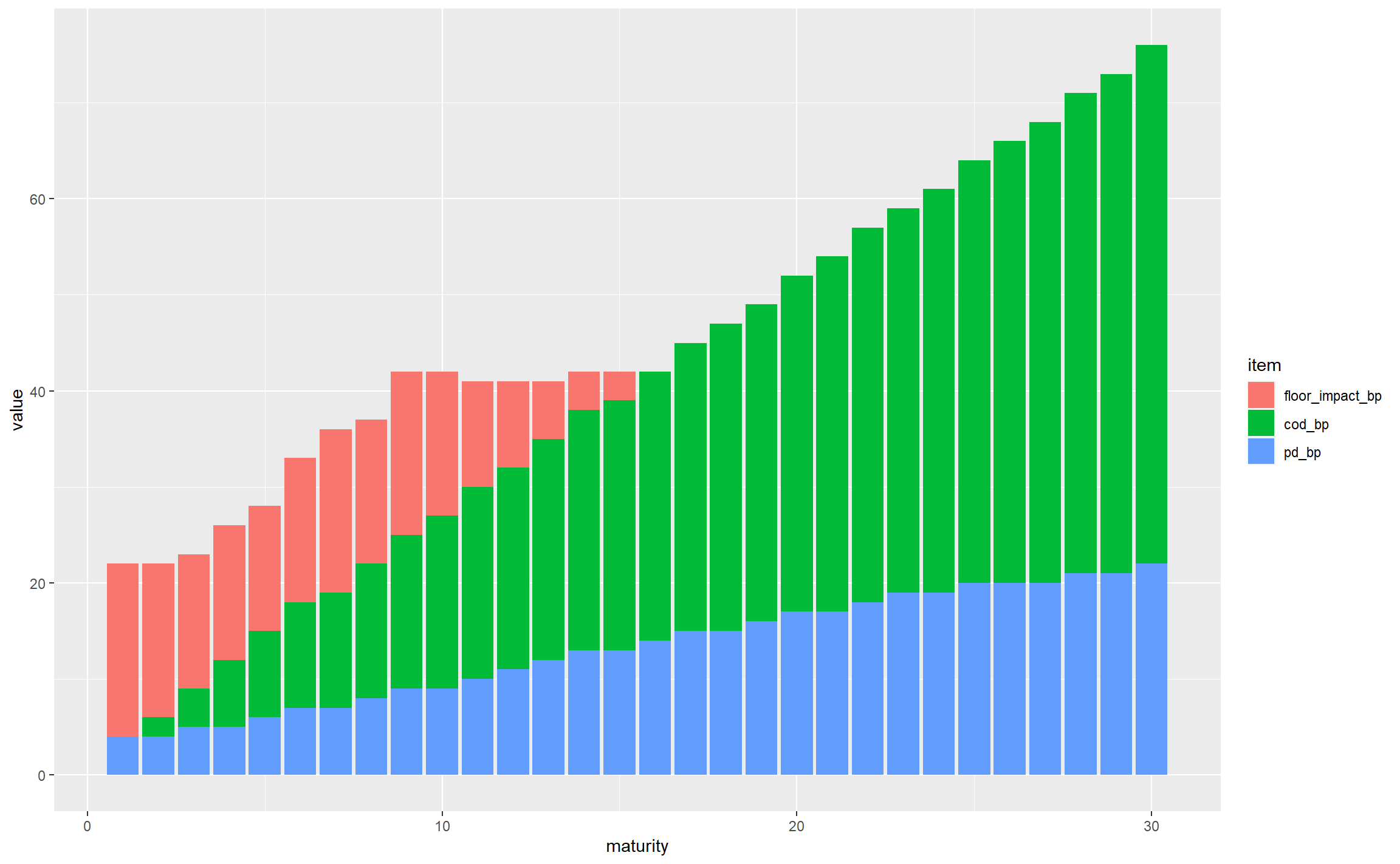
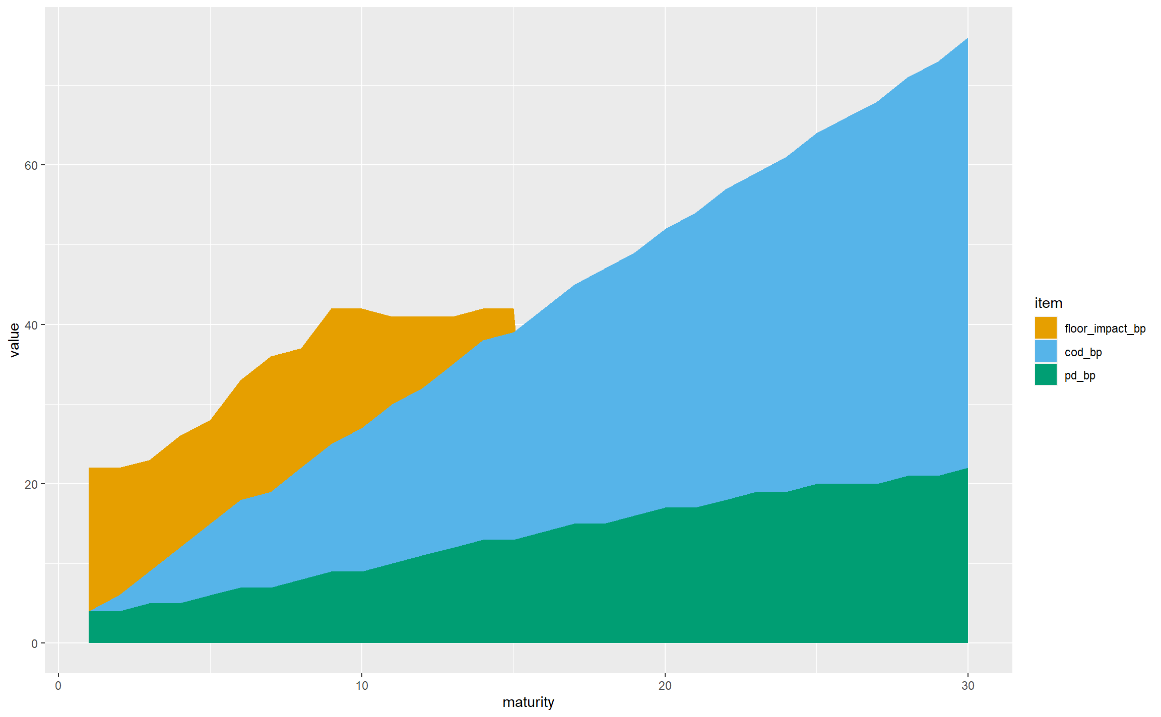
This is off to a decent start; for non-financial CQS2 assets we can see that:

  • the total FS varies significantly by maturity, from around 20bps to nearly 80bps
  • the PD starts small and rises with maturity, as expected (longer duration bonds have more probability of default, and this outweighs the impact of expressing the resulting expected losses as an annualised basis points value)
  • the CoD has a similar general shape, following similar logic (longer-maturity bonds have more downgrade risk even when annualised)
  • the floor bites in the first 14 years, but seems to flatten out, and gets overtaken by the sum of PD and CoD at longer maturities
  • looking across all maturities, CoD is the dominant contributor

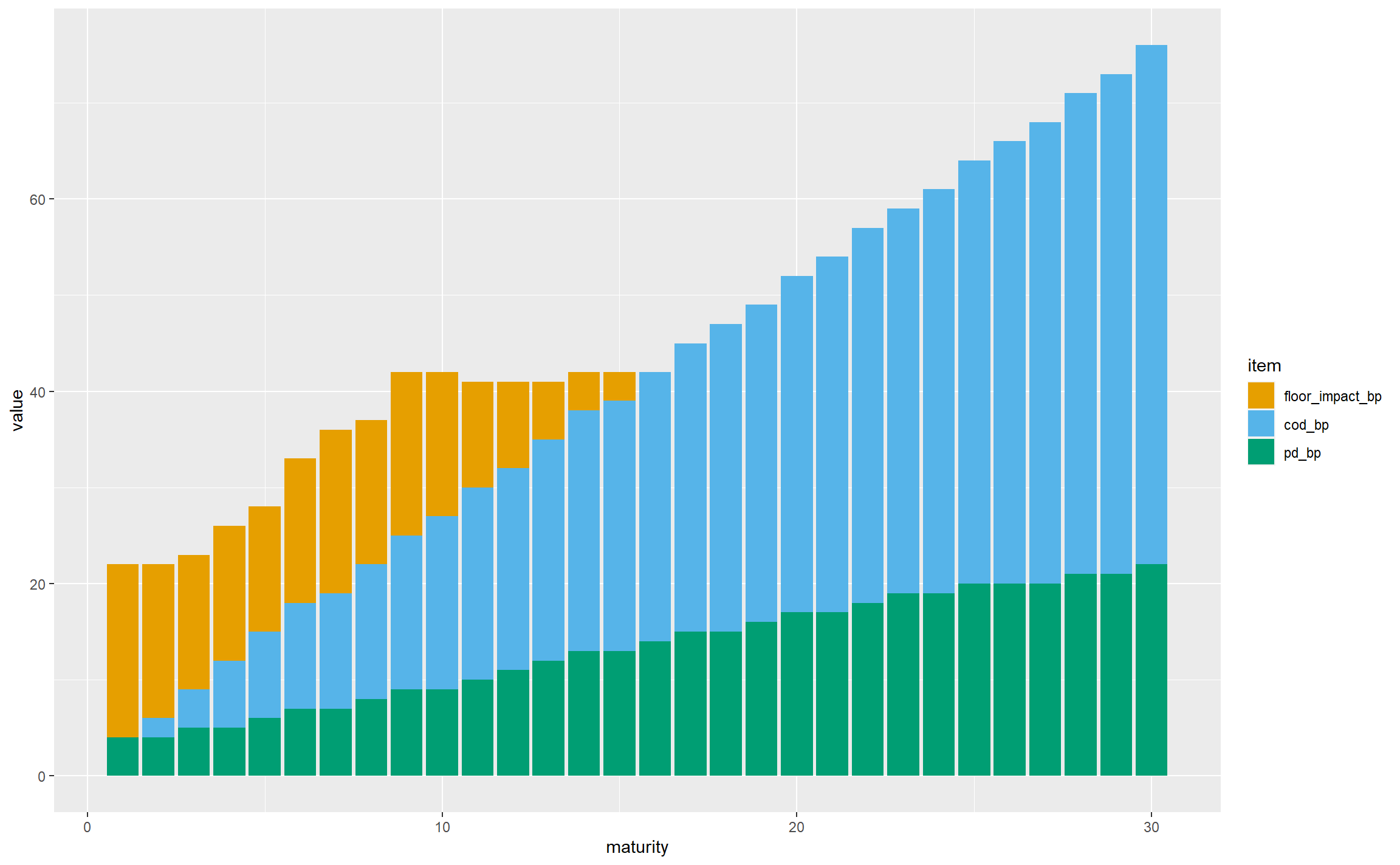
There are a few things to do with tidying up axis titles and so on, but the first thing we should do is choose colours that are visible to colour-blind people – the default red and green colours used by ggplot may not be very distinguishable. Here we’re using the colours put forward by Wong.

safe_colours <- c("#E69F00", "#56B4E9", "#009E73")
ggplot(gbp_fs_for_single_plot, aes(x = maturity, y = value, fill = item)) +
  geom_col() +
  scale_fill_manual(values = safe_colours)

Having dealt with the colours, let’s develop the geometry. There are a lot of columns, so moving to a stacked area chart would be visually simpler, and the key observations can still be drawn:

ggplot(gbp_fs_for_single_plot, aes(x = maturity, y = value, fill = item)) +
  geom_area() +
  scale_fill_manual(values = safe_colours)

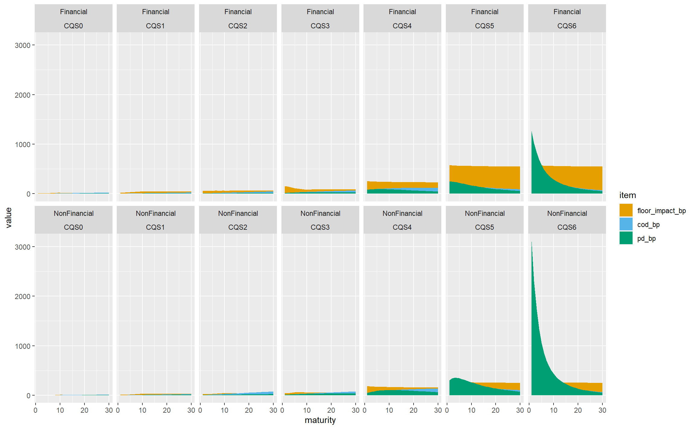
Now let’s bring in CQS and sector. This chart is already complicated enough without adding more areas to it, so we’re going to need a different technique. ggplot supports faceting, where the data is split into subsets shown in different panels with the same general structure. Here we are going to facet by CQS and sector, and this is trivial to achieve in ggplot, much more so than it would be in Excel, say:

ggplot(gbp_fs_for_plot, aes(x = maturity, y = value, fill = item)) + # Note using all the data now
  geom_area() +
  scale_fill_manual(values = safe_colours) +
  facet_wrap(~sector + CQS, nrow = 2)

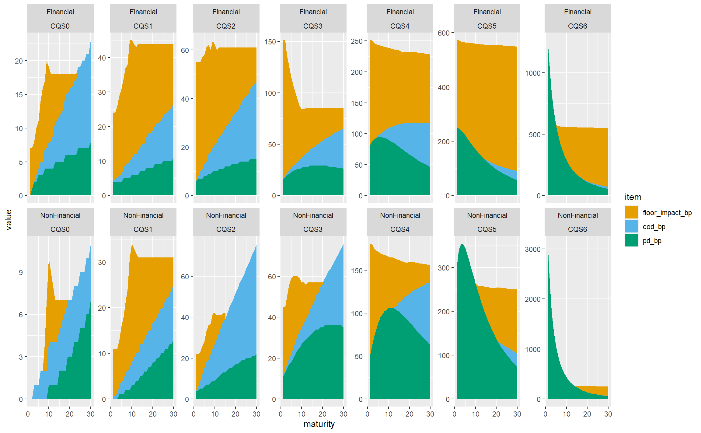
If we’re very charitable, this does achieve the goal of showing all the data and allowing the relationships between CQSs and sectors to be seen, but clearly it is visually dominated by the very large PD for CQS6 non-financial assets, and not much use at all. We can remedy this by allowing the y-axis scales to vary independently on each panel:

ggplot(gbp_fs_for_plot, aes(x = maturity, y = value, fill = item)) +
  geom_area() +
  scale_fill_manual(values = safe_colours) +
  facet_wrap(~sector + CQS, nrow = 2, scales = "free_y")

This is much more informative, at the cost of viewers needing to pay careful attention to the y-axis scales. To pick out just a few observations:

  • The floor bites almost all the time for financial sector bonds, and is less dominant in the non-financial sector. We might hypothesise that this reflects the very high spreads seen in the financial sector in the 2008-2009 credit crisis.
  • CoD is less dominant for lower-rated bonds (CQS4 and below) as they are already low-quality and the scope for downgrading is less than for higher-rated bonds.
  • PD is not monotone with maturity for lower-rated bonds, presumably because the annualisation effect in the basis point values outweighs the increase in the underlying expected losses.

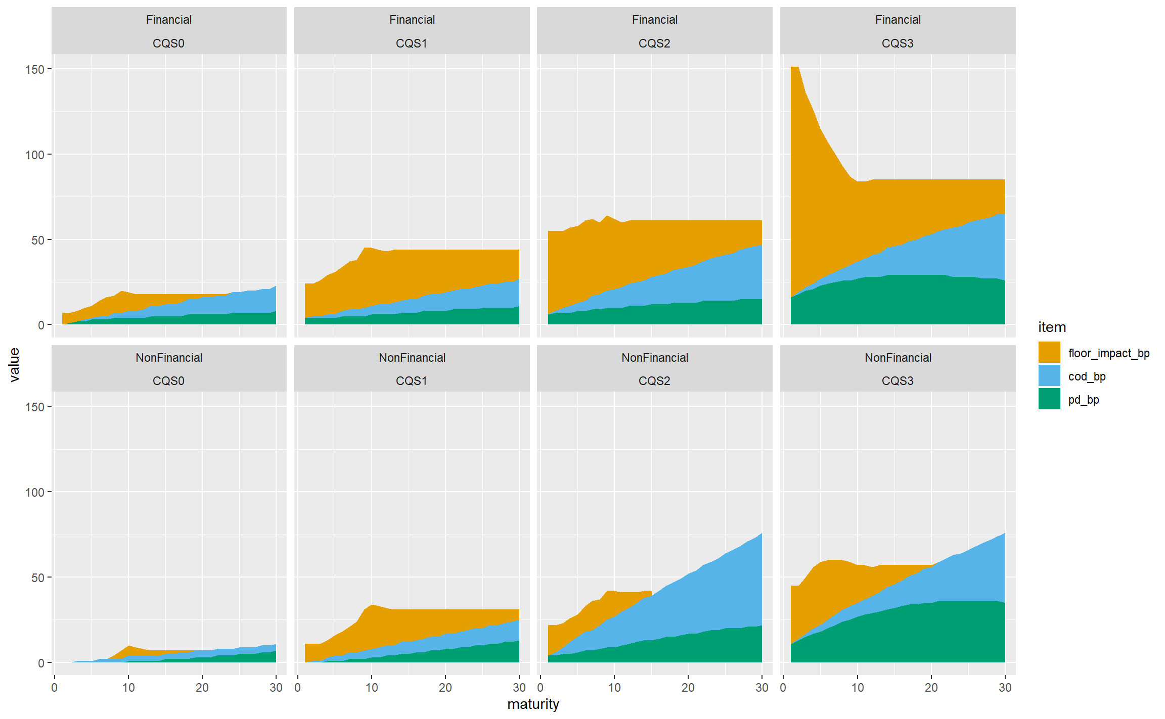
In practice, life insurers don’t hold much in the way of sub investment grade bonds, and we wouldn’t lose that much by restricting the chart to CQS0-CQS3 assets, which gives less for viewers to try to take in:

gbp_fs_ig_only <- subset(gbp_fs_for_plot, CQS %in% c("CQS0", "CQS1", "CQS2", "CQS3"))
ggplot(gbp_fs_ig_only, aes(x = maturity, y = value, fill = item)) + 
  geom_area() +
  scale_fill_manual(values = safe_colours) +
  facet_wrap(~sector + CQS, nrow = 2, scales = "free_y")

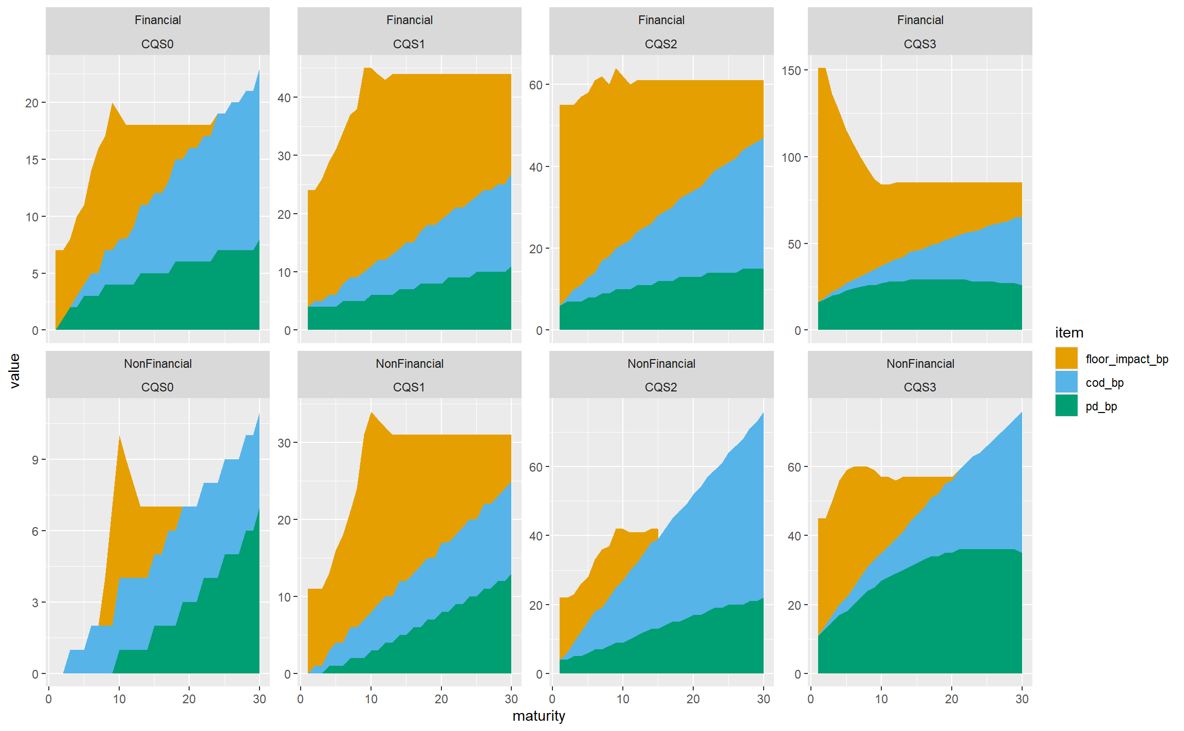
Let’s try reverting to a fixed y-axis scale, which allows the variability in the total FS across CQSs and sectors to be seen more readily, at the cost of de-emphasising the structure within each panel:

ggplot(gbp_fs_ig_only, aes(x = maturity, y = value, fill = item)) + 
  geom_area() +
  scale_fill_manual(values = safe_colours) +
  facet_wrap(~sector + CQS, nrow = 2)

That’s not bad, so let’s stop there in terms of the structure of the plot, and tidy it up a bit.

  • Since we’re not using free y-axis scales, we can use facet_grid instead of facet_wrap. This removes the repetition of the sector and CQS labels. (It isn’t possible to have free scales with facet_grid.)
  • Add more breaks on the axes: every 5 years on the x-axis and 20bps on the y-axis.
  • Add a title, caption and axis titles.
  • Remove the title of the legend (‘item’) which doesn’t add anything useful.
  • Rename the legend labels to be less technical.
  • Change the font sizes to be more readable.
ggplot(gbp_fs_ig_only, aes(x = maturity, y = value, fill = item)) +
  geom_area() +
  scale_fill_manual(values = safe_colours,
                    labels = c("Floor Impact", "CoD", "PD")) +
  scale_x_continuous(breaks = 5 * 0:6) +
  scale_y_continuous(breaks = 20 * 0:8) +
  facet_grid(rows = vars(sector), cols = vars(CQS)) +
  labs(title = "Breakdown of Fundamental Spreads for investment-grade corporate bonds at 31 December 2019",
       caption = "Source: EIOPA") +
  xlab("Maturity") + ylab("FS item (basis points)") +
  theme(legend.title = element_blank(),
        plot.title = element_text(size = 16),
        plot.caption = element_text(size = 12),
        axis.title = element_text(size = 14),
        axis.text =  element_text(size = 12),
        strip.text = element_text(size = 14),
        legend.text = element_text(size = 14))

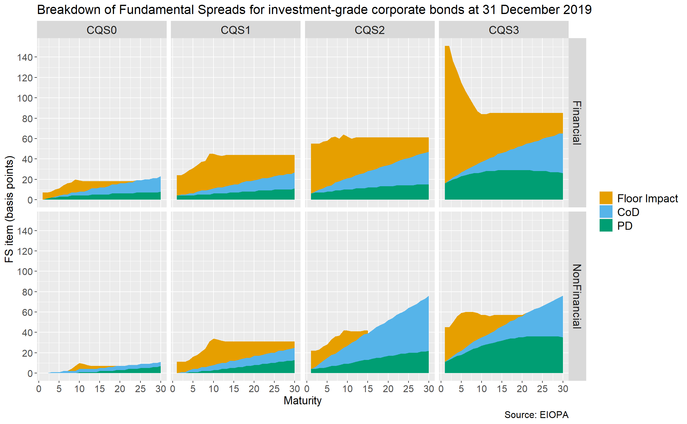
As is often the case with ggplot, the code to tidy the chart up is longer than the code for the overall structure!

Summary

In this post, we discussed the structure and granularity of the EIOPA FS, and showed how to download a particular set of published values and extract this from Excel to R. We then manipulated the data so it could be plotted, and explored different plotting approaches.

Categories
General

Delivering at different scales

I spent several years as a ‘traditional contractor’ through my previous consultancy. The ‘traditional’ model was to take on full-time contracts for several months with a main client, possibly with some smaller contracts as well. There is definitely still a market for that kind of approach, and Polynya is very happy to work with clients on that basis.

However, in renewing ties with old friends and colleagues in the independent consulting market, and exploring new opportunities, it’s become clear that the traditional approach is in the middle of a spectrum.

At the smaller-scale end of that spectrum, I’ve had discussions with clients about performing a targeted review. For example, some firms are interested in expertise and challenge on specific aspects of forthcoming Internal Model major change applications. The duration is a week or two, and the deliverable a report with recommendations about how the approach, or its documentation and presentation to the PRA, can be refined.

The relatively small scale of the engagement doesn’t detract from the core purpose of using expertise and experience to help the client achieve its objectives. It also builds knowledge of the client’s business, and working relationships with its staff, giving a potential springboard for further mutually beneficial engagements.

At the other end of the spectrum are much larger projects. One approach here is to engage a ‘Big 4’ consulting firm, and there are clearly cases where this remains very sensible. However, where very specific expertise is needed, the Big 4 aren’t always in the best position to provide it. And engaging multiple independent contractors comes with an overhead to the client to coordinate their delivery.

Many independent contractors – and I am no exception – thrive on the independence. But we only make a living by delivering value to clients through our expertise and experience. A middle path is for independent consultants to join forces with each other through ‘collectives’, while retaining their independent identities. This enables delivery at scale, with the collective coordinating its own activities. And even though the expertise is much more focused, the pricing is nowhere near Big 4 levels.

So I’m delighted to report that Polynya has joined the R Calc collective of credit risk experts, led by Leigh Baker. Across the collective we have deep knowledge of credit risk from multiple industries, and look forward to bringing that pooled expertise to bear for clients’ benefit. Whether that’s life insurers who are looking to widen their range of credit assets, or banks and building societies who would benefit from a breadth of expertise not just with mainstream lending, but also with more specialised products like equity release and retirement interest-only mortgages, R Calc stands ready to assist.

In conclusion, Polynya is pleased to assist clients at a wide range of scales, from targeted reviews, through traditional contracting, to participation within collectives. Please contact us if you’d like to discuss how we can help.

Categories
R

Using R Markdown with WordPress

R Markdown

Markdown is a simple formatting syntax for writing HTML, PDF, and Microsoft Word documents.

R Markdown is Markdown interwoven with chunks of R code. This enables the results of calculations and analyses, and equations, plots, diagrams and other graphics, to be embedded within the output, and supports reproducible research.

Put differently, an R Markdown document is a record of an analysis that both contains the code needed to reproduce it, and commentary that enables it to be understood. This is very much more practical and auditable than running scripts and copying isolated results into a separate document.

For more details on using R Markdown see http://rmarkdown.rstudio.com and this cheat sheet.

WordPress

WordPress is a platform for building websites and blogs. This site uses WordPress technology but is hosted separately to https://wordpress.com/.

It is possible to take HTML output from R Markdown and manually upload this to WordPress, but this is somewhat tedious and error-prone, for example any plots would need to be uploaded separately. So I started looking for a more streamlined approach. It took three attempts to find an approach that did what I was looking for – I outline the first two briefly for completeness and discuss the third in detail.

Attempt 1: RWordPress package

A quick web search led to a blog post talking about the RWordPress package. This is on GitHub rather than CRAN.

RWordPress is used by the knitr function knit2wp but at the time of writing this post, RWordPress was last updated in 2012 and uses the XMLRPC API to connect to WordPress. This API needs to be used with caution as it has potential security issues.

Further, RWordPress relies on the RCurl package. On Windows 10 this uses an outdated version of the underlying OpenSSL library that does not support modern encryption techniques, as noted in an RWordPress GitHub issue. I received an error message about an SSLv3 alert handshake failure that I couldn’t resolve.

Attempt 2: wordpressr package

Further searching located the wordpressr package, which is on CRAN. This uses the WordPress REST API which is less of a security concern than XMLRPC.

The functionality in wordpressr allows posts to be created from R, and I got this to work fairly easily, but it requires the HTML to be supplied directly, and doesn’t have the integration with R Markdown that I was looking for.

Attempt 3: goodpress package

Finally I found a blog post talking about the goodpress package. goodpress is under development at the time of writing this post, but uses the REST API, has decent integration with R Markdown, and did everything I wanted.

There are helpful instructions for setting up goodpress here, expanded upon somewhat here. To summarise, the steps involved are:

  1. Install the Application Passwords plugin. This allows authentication for the REST API under a new password that is distinct from the WordPress password for the site itself. For additional security it is possible to create a separate user with Editor rights and associate the application password with that user rather than the main admin user.
  2. Create a new application password from the Users part of the WordPress dashboard by following the instructions under Creating Application Password Manually here.
  3. Add additional CSS to WordPress for syntax highlighting. See the instructions here.
  4. Add two entries to the .Renviron file to create environment variables WP_USER and WP_PWD. WP_USER is set to the actual user ID, not the name created the application password under (e.g. rmarkdown). WP_PWD is set to the application password generated in step 2. goodpress uses the values from the environment variables and in the version at the time of writing, cannot be configured to accept values from elsewhere. For background, the .Renviron file is used to set up environment variables accessible to R and RStudio. It needs to be saved under the ‘home’ directory, which can be found by executing path.expand("~") in the R console. Saving the user name and password in environment variables reduces the risk of accidentally sharing them, for example if the R Markdown files are committed to git or another source control system. It also provides a single point of change if it’s necessary to revoke the application password or change it from time to time.
  5. Install the goodpress package using devtools::install_github("maelle/goodpress", ref = "main"). This is likely to install various dependencies.
  6. Create a folder to hold the R Markdown document and intermediate files produced by goodpress. The author of goodpress suggests one folder per post, which seems sensible.
  7. Create a skeleton R Markdown document in the newly-created folder. goodpress needs this to be called index.Rmd and again this name cannot yet be changed. The header of the R Markdown document needs to be closely aligned to the examples provided in the goodpress documentation for wp_post. In particular use output: hugodown::md_document rather than output: html_document. This makes knitr produce an .md file in ‘Hugo’ format, a Markdown dialect that goodpress is able to interpret and load to WordPress. It is also sensible to say status: "draft" to allow the post to be previewed and if necessary edited in WordPress before it is published and visible on the Web. goodpress takes care of creating categories and tags used in the R Markdown header.
  8. Write the R Markdown document as usual.
  9. Use knitr via the Knit button in RStudio to produce a Markdown document (index.md) from the R Markdown document (index.Rmd) and an HTML preview. This won’t look exactly the same as on the site, because of CSS differences, for example, but is still useful for proof-reading purposes.
  10. In a separate script (I suggest calling it submit.R), set up a single line of R code of the form goodpress::wp_post("<folder holding the .Rmd and .md files>", "<root URL of the site e.g. https://www.polyact.co.uk>") and execute this line in the R console to create the draft post in WordPress. If all goes well the message Post posted with status draft will be shown.
  11. Go into Posts in the WordPress Dashboard to preview or edit the newly-created post.
  12. It is possible to amend the R Markdown, re-knit and re-post to WordPress – goodpress takes care of creating the post the first time and editing it thereafter.

Equations

Provided MathJax is set up on the WordPress site, for example using the Simple MathJax plugin, mathematical expressions in LaTeX syntax within the R Markdown document will be rendered properly in posts. To prove the concept, a simple inline expression is \((a+b)^2 + \int_a^b{x^2 \mathrm{d}x}\), producing using the LaTeX code $(a+b)^2 + \int_a^b{x^2 \mathrm{d}x}$.

‘Display’ expressions are also supported, for example Euler’s Identity: \[ e^{i\pi} + 1 = 0 \]

Plots

A very useful feature of goodpress is capturing the image files that hold the result of plotting, uploading these to the site’s WordPress media library, and linking them into the post. This ‘just worked’ when I tried it, and didn’t need any further configuration.

Plots can be produced using the built-in R plotting system, here a very simple plot of the built-in pressure dataset:

plot(pressure)

ggplot2 is also supported. This simple example uses the diamonds dataset and shows how the price of diamonds (on the y-axis) varies with the number of carats (on the x-axis), the diamond cut quality (the colour of the points) and diamond clarity (the facets).

ggplot(diamonds, aes(x=carat, y=price, color=cut)) +
  geom_point() +
  facet_wrap(~ clarity)

Conclusion

The goodpress package is a very helpful way of allowing blog posts to be created from R Markdown documents. There is some initial set-up to be done, but the overhead is modest in relation to the time saved by not needing to manually upload image files. Future technical posts on this site will use goodpress.

Categories
General

Why Polynya?

Polynya is a loanword from Russian, meaning an area of open water surrounded by sea ice, particularly in the Arctic. As such, it is a base from which to explore the hidden depths of icebergs, and a metaphor for the insights arising from risk modelling.

We shortened it for the website after receiving very sound advice from a friend – ‘don’t choose a name that’s hard to spell’ – and this gives it an appealingly mathematical air. (Take cross-language mathematical puns where you can, they don’t come along all that often!)